Gravity map and data of the eastern half of the Big Bear Lake 100,000 scale quadrangle, California and analysis of the depths of several basins.

Frequently anticipated questions:

• What does this data set describe?
  1. How might this data set be cited?
  2. What geographic area does the data set cover?
  3. What does it look like?
  4. Does the data set describe conditions during a particular time period?
  5. What is the general form of this data set?
  6. How does the data set represent geographic features?
  7. How does the data set describe geographic features?
• Who produced the data set?
  1. Who are the originators of the data set?
  2. Who also contributed to the data set?
  3. To whom should users address questions about the data?
• Why was the data set created?
• How was the data set created?
  1. From what previous works were the data drawn?
  2. How were the data generated, processed, and modified?
  3. What similar or related data should the user be aware of?
• How reliable are the data; what problems remain in the data set?
  1. How well have the observations been checked?
  2. How accurate are the geographic locations?
  3. How accurate are the heights or depths?
  4. Where are the gaps in the data? What is missing?
  5. How consistent are the relationships among the data, including topology?
• How can someone get a copy of the data set?
  1. Are there legal restrictions on access or use of the data?
  2. Who distributes the data?
  3. What's the catalog number I need to order this data set?
  4. What legal disclaimers am I supposed to read?
  5. How can I download or order the data?
• Who wrote the metadata?

What does this data set describe?

1. How might this data set be cited?
   Roberts, C.W., Jachens, R.C., Katzenstein, A., Smith, G.A, and Johnson, R., 2002, Gravity map and data of the eastern half of the Big Bear Lake 100,000 scale quadrangle, California and analysis of the depths of several basins.: U.S. Geological Survey Open-File Report 02-353, U.S. Geological Survey, Menlo Park, California.

   Online Links:

   • http://pubs.usgs.gov/of/2002/0353/

2. What geographic area does the data set cover?

   West_Bounding_Coordinate: -116.500
   East_Bounding_Coordinate: -116.000
   North_Bounding_Coordinate: 34.500
   South_Bounding_Coordinate: 34.000
   

3. What does it look like?

   http://pubs.usgs.gov/of/2002/0353/images/index.gif (GIF)

   Index map showing field location within state of California, 411x309 pixels, 3k bytes.

   http://pubs.usgs.gov/of/2002/0353/images/gravity-thumb.jpg (GIF)

   Reduced-size, color contoured isostatic gravity map, 782x936 pixels, 116k bytes

4. Does the data set describe conditions during a particular time period?

   Calendar_Date: 2002

   Currentness_Reference:

   publication date

5. What is the general form of this data set?

   Geospatial_Data_Presentation_Form: map
   

6. How does the data set represent geographic features?
   1. How are geographic features stored in the data set?
      This is a point data set.
   2. What coordinate system is used to represent geographic features?
      Horizontal positions are specified in geographic coordinates, that is, latitude and longitude. Latitudes are given to the nearest 0.01 minute. Longitudes are given to the nearest 0.01 minute. Latitude and longitude values are specified in Degrees and decimal minutes. The horizontal datum used is North American Datum of 1927.
      The ellipsoid used is Clarke 1866.
      The semi-major axis of the ellipsoid used is 6378206.4.
      The flattening of the ellipsoid used is 1/294.98.
      

      Vertical_Coordinate_System_Definition:

      Altitude_System_Definition:

      Altitude_Datum_Name: National Geodetic Vertical Datum 1929 (NGVD29)
      Altitude_Resolution: 0.1
      Altitude_Distance_Units: feet
      Altitude_Encoding_Method: Attribute values
      

7. How does the data set describe geographic features?

   (table row)

   Gravity observation. Attribute labels here were made up by the metadata editor; they do not appear in the data file.

   (stname)

   Station name (columns 1- 8 type A8) Identifier without scientific significance

   (latdeg)

   Degrees of latitude (columns 10-11 type I2)

   Value	Definition
   34

   (latmin)

   Hundredths of minutes of latitude (columns 12-15 type I4)

   Range of values
   Minimum:	59
   Maximum:	2980
   Units:	minutes / 100
   Resolution:	1

   (londeg)

   Degrees of longitude (columns 17-19 type I3)

   Value	Definition
   116

   (lonmin)

   Hunderedths of minutes of longitude (columns 20-23 type I4)

   Range of values
   Minimum:	2
   Maximum:	2920
   Units:	minutes / 100
   Resolution:	1

   (elevft)

   Elevation, in tenths of feet (columns 24-29 type I6)

   Range of values
   Minimum:	17317
   Maximum:	55338
   Units:	feet / 10
   Resolution:	1

   (obsgrav)

   Observed gravity, in hundredths of mGal, without leading 9 (columns 30-36 type I7)

   Range of values
   Minimum:	7921220
   Maximum:	7948170
   Units:	mGal / 100
   Resolution:	1

   (acc1)

   General elevation and location code

   Value	Definition
   (no value)
   P	On or near surveyed mark

   (acc2)

   Elevation code

   Value	Definition
   (no value)
   3	Transit or good alidade survey: 1.0 ft, 0.06 mGal

   (acc3)

   Latitude code

   Value	Definition
   (no value)
   2	Location known to 0.04 in on 1:24,000 map: 0.014 min, 84 ft, 0.02 mGal

   (acc4)

   Observed gravity code

   Value	Definition
   (no value)
   3	Average LaCoste and Romberg or multiple Worden meter: 0.05 mGal

   (faa)

   Free-air anomaly, in hundredths of mGal (columns 41-46 type I6)

   Range of values
   Minimum:	-4964
   Maximum:	8139
   Units:	mGal / 100
   Resolution:	1

   (sba)

   Simple Bouguer anomaly, in hundredths of mGal (columns 47-52 type I6)

   Range of values
   Minimum:	-11950
   Maximum:	-7559
   Units:	mGal / 100
   Resolution:	1

   (iztc)

   Inner-zone terrain correction, in hundredths of mGal (columns 53-57 type I5)

   Range of values
   Minimum:	0
   Maximum:	226
   Units:	mGal / 100
   Resolution:	1

   (tc)

   Total terrain correction, in hundredths of mGal (columns 58-62 type I5)

   Range of values
   Minimum:	42
   Maximum:	1275
   Units:	mGal / 100
   Resolution:	1

   (tccode)

   Terrain correction code denoting extent of inner-zone terrain correction and system: upper case denotes Hayford-Bowie system of zones, lower case denotes Hammer system of zones. Z, computer calculated from 0.0-0.59 km (column 63 type A1)

   Value	Definition
   (no value)
   D	(from Hayford-Bowie system of zones)
   g	(from Hammer system of zones)
   h	(from Hammer system of zones)

   Formal codeset
   Codeset Name:	Hayford-Bowie system of zones (for upper-case letter codes)
   Codeset Source:	Hayford, J.F., and Bowie, William, 1912, The effect of topography and isostatic compensation upon the intensity of gravity: U.S. Coast and Geodetic Survey Special Publication no. 10, 132 p.

   Formal codeset
   Codeset Name:	Hammer system of zones (for lower-case letter codes)
   Codeset Source:	Hammer, Sigmund, 1939, Terrain corrections for gravimeter stations: Geophysics, v. 4, p. 184-194.

   (cba)

   Complete Bouguer anomaly reduced for a density of 2.67 g/cc, in hundredths of mGal (columns 64-69 type I6)

   Range of values
   Minimum:	-11850
   Maximum:	-7392
   Units:	mGal / 100
   Resolution:	1

   (ia)

   Isostatic gravity anomaly reduced for a density of 2.67 g/cc, in hundredths of mGal (columns 70-75 type I6)

   Range of values
   Minimum:	-3549
   Maximum:	1093
   Units:	mGal / 100
   Resolution:	1

   (comment)

   Comment (columns 76-80 type A4)

   Value	Definition
   (no value)
   ISOW	isostatic correction made for the whole earth

Who produced the data set?

1. Who are the originators of the data set? (may include formal authors, digital compilers, and editors)
   • Roberts, C.W.
   • Jachens, R.C.
   • Katzenstein, A.
   • Smith, G.A
   • Johnson, R.
2. Who also contributed to the data set?
3. To whom should users address questions about the data?
   Carter Roberts

   U.S. Geological Survey

   345 Middlefield Rd, MS 989

   Menlo Park, CA
   

   U.S.A.

   650-329-5319 (voice)

   croberts@usgs.gov

Why was the data set created?

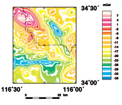
This gravity dataset was collected in order to have adequate gravity information over the basins and adjacent basement rocks that the gravity data could be inverted to separate the basin component and then the thickness of the basins could be computed.

How was the data set created?

1. From what previous works were the data drawn?
2. How were the data generated, processed, and modified?

   Date: 1986 (process 1 of 3)

   Gravity measurements were made at more than 1200 locations by the authors and their assistants. Combined with older data this gives more than 2300 data points used for the gravity map of the 30 by 30 minute quadrangle.
   We wish to thank Roberts Voorhies, MCAGCC 29 Palms for assistance with access to do the survey, especially in the Range areas and Dennis Clark, USGS San Diego, for providing the well information that was vital for the depth to basement computation.
   All gravity data were reduced using standard gravity corrections, including: (a) the earth tide correction, which corrects for tidal effects of the moon and sun; (b) instrument drift correction, which compensates for drift in the instrument's spring; (c) the latitude correction, which incorporates the variation of the Earth's gravity with latitude; (d) the free-air correction, which accounts for the variation in gravity due to elevation relative to sea level; (e) the Bouguer correction, which corrects for the attraction of material between the station and sea level; (f) the curvature correction, which corrects the Bouguer correction for the effect of the Earth's curvature; (g) the terrain correction, which removes the effect of topography to a radial distance of 166.7 km; and (h) the isostatic correction, which removes long-wavelength variations in the gravity field inversely related to topography.
   Conversion of LaCoste and Romberg gravity meter readings to milligals was made using factory supplied calibration constants and a secondary calibration factor determined from multiple gravity readings over the high-precision Mt. Hamilton calibration loop east of San Jose, Calif. (Barnes and others, 1969). Observed gravity values were based on a time-dependant linear drift between successive base readings and were referenced to the International Gravity Standardization Net 1971 (IGSN 71) gravity datum (Morelli, 1974, p. 18). The primary base station was PBB8 (Roberts and Jachens 1986) south of Twentynine Palms where the observed gravity is 979,396.28 mGal (9.7939628 m/sec2). Free-air gravity anomalies were calculated using the Geodetic Reference System 1967 formula for theoretical gravity on the ellipsoid (International Union of Geodesy and Geophysics, 1971, p. 60) and Swick's formula (1942, p. 65) for the free-air correction. Bouguer, curvature, and terrain corrections were added to the free-air correction to determine the complete Bouguer anomaly at a standard reduction density of 2.67 g/cm3.
   Locations for most of the new stations released here for the first time were obtained either with conventional surveying equipment or a differential GPS system with most positions determined in real time.
   Terrain corrections, which account for the variation of topography near a gravity station, were computed using a three-part process: the innermost or field terrain correction, inner-zone terrain correction, and outer-zone terrain correction. The innermost or field terrain correction was estimated in the field, using a system of tables and charts, and typically extends to a radial distance of 53 or 68 m, Hammer (1939) zone C or Hayford and Bowie (1912) zone B, respectively.
   Inner-zone terrain corrections were styled after the Hayford and Bowie (1912) system that divide the terrain surrounding a gravity station into zones and equal area compartments. For all the newer stations average elevations for each compartment were computed from a detailed digital elevation model (DEM) derived from USGS 7.5 minute DEMs with a resolution of 30 m. Inner-zone terrain corrections typically extended to a radial distance of 0.59 km, Hayford and Bowie (1912) zone D. Terrain corrections were then calculated based on the average estimated elevation of each compartment (Spielman and Ponce, 1984).
   Outer-zone terrain corrections, to a radial distance of 166.7 km, were computed using a DEM derived from USGS 1:250,000-scale topographic maps and an automated procedure (Plouff, 1966; Plouff, 1977; Godson and Plouff, 1988). Digital terrain corrections are calculated by computing the gravity effect of each grid cell using the distance and difference in elevation of each grid cell from the gravity station.
   Finally, a regional isostatic gravity field was removed from the Bouguer field assuming an Airy-Heiskanen model for isostatic compensation of topographic loads (Jachens and Roberts, 1981). An assumed crustal thickness of 25 km, a crustal density of 2.67 g/cm3, and a density contrast across the base of the model of 0.4 g/cm3 was used and the computation was carried out for topography averaged over 3 by 3 minute compartments to a distance of 166.7km from each station. Isostatic and terrain corrections beyond that distance were interpolated from a grid generated from Karki et al. (1961).
   Principal facts of the gravity data are available on the Get Data page. Gravity values are expressed in milligals (mGal), a unit of acceleration where 1 Gal equals 1 cm/sec2.
   Depth to basement computation method
   With a gravity data set and the surface distribution of basement rocks it becomes possible to compute possible basin configurations.
   The procedure begins with a computer program that attempts to separate the residual gravity field into two components, a basement component and a basin component. All gravity measurements located on pre-Cenozoic rocks are considered to be on basement. Wells that penetrate basement are used as depth control points.
   An isostatic residual gravity grid and several files of gravity stations are input along with a mask grid that shows areas considered basement. We have made sure that there is at least 100 meters from any basement gravity station to the nearest area in the grid designated as basin since the program sometimes has trouble when a basement station is on the edge of a basin. The mask grid was made using geolgy from Dibblee (1967, 1968) and Moyle (1984).
   A density contrast versus depth model based on any available density information is used by the program. For the Surprise Spring area numerous wells that penetrated basement rocks were available to constrain the computed depths. In the Deadman Lake Basin and the Joshua Tree Basin the only wells penetrating the basement rocks are near the margins so the total depth is uncertain although a variety of different models give similar configurations and relative depths.
   The method used in this study to estimate the thickness of Cenozoic rocks is an updated version of the iterative method developed by Jachens and Moring (1990) that incorporates drill hole and other geophysical data (B. Chuchel, U.S. Geological Survey, written communication, 1996). The method requires knowledge of the residual gravity field, of the exposed geology, and of the vertical density variation within the Cenozoic basin deposits. Data from drill holes that penetrate the basement surface (defined to be pre-Cenozoic in age) and any other geophysical data that provide constraints on the thickness of the basin fill are also used.
   The method separates the gravity field into two components, that which is caused by variations of density within the pre-Cenozoic bedrock and that which is caused by variations of thickness of the Cenozoic basin fill. To accomplish this process, the gravity data are separated into observations made on bedrock outcrops and observations made on Cenozoic deposits. The second set of observations is inverted, using a density-depth function estimated to characterize the Cenozoic deposits, to yield the thickness of Cenozoic deposits. The inversion is complicated by two factors: (1) bedrock gravity stations are influenced by the gravity anomaly caused by low-density deposits in nearby basins, and (2) the bedrock gravity field varies laterally because of density variations within the bedrock. The inversion presented here does not take into account lateral variations in the density distribution of the Cenozoic deposits.
   To overcome these difficulties, a first approximation of the bedrock gravity field is determined by interpolating a smooth surface through all gravity values measured on bedrock outcrops. Bedrock gravity values are also calculated at locations where drill holes penetrated bedrock using the Cenozoic density-depth function. The basin gravity is then the difference between the observed gravity field on the original map and the first approximation of the bedrock gravity field and is used to calculate the first approximation of the thickness of Cenozoic deposits. The thickness is forced to zero where bedrock is exposed.
   This first approximation of the bedrock gravity is too low near the basin edges because of the effects of the nearby low-density deposits on the bedrock stations. The bedrock gravity station values are "corrected" for the effects of the low-density deposits (the effects are calculated directly from the first approximation of the thickness of the Cenozoic deposits) and a second approximation of the bedrock gravity field is made by interpolating a smooth surface through the corrected bedrock gravity observations. This iteration leads to an improved estimate of the basin gravity field, an improved depth to bedrock, and a new correction to the bedrock gravity values. This procedure is repeated until successive iterations produce no significant changes in the bedrock gravity field. We have checked the computed basin thickness against wells that are known to not penetrate the basement rocks. We have also made runs without some of the constraining wells to see that the resulting thicknesses and configurations are not dramatically different.
   Use of this method at Yucca Flat Nevada where there are an extremely large number of wells (Phelps et al. 1999) showed that the procedure operating with some of the wells can produce a reasonable approximation of the true basement surface as determined by all the wells. These results in a basin with exceptional well control suggest that the method is very good at predicting the shape of the basin but may not produce precisely the magnitude of basin thickness.
   Lateral variations in basin fill density, unless abrupt, would not change the overall general shape of the basin as predicted by the method.
   The method has several inherent limitations:
   (a) In some areas the distribution of basement gravity stations is not ideal due to the large areas covered by later deposits or the difficulty of reaching the basement rocks to obtain measurements.
   (b) The distribution, depths and density or litholigic information from wells is usually less than ideal. In deeper basins wells seldom penetrate basement rocks. Well logs may be unreliable. Some wells that claim to penetrate basement rocks may not do so. Several logs in the Joshua Tree Basin show alternating basement and sedimentary rocks. One well that claimed to bottom in "granite" was later deepened and passed through another zone of "sandstone."
   (c) The process assumes it is dealing with a basin and must satisfy the gravity field between the ground surface and the basement surface. It can not model any density variations below the bedrock surface.
   (d) While different density-depth functions can be used in different area, a sharp step appears where the change occurs. The results from the program may also be affected slightly by the grid spacing.
   References cited
   Barnes, D.F., Oliver, H.W., and Robbins, S.L., 1969, Standardization of gravimeter calibrations in the Geological Survey: Eos, Transactions, American Geophysical Union, v. 50, no. 10, p. 626-627.
   Biehler, Shawn, Tang, R.R., Ponce, D.A., and Oliver, H.W., 1988, Bouguer gravity map of the San Bernardino Quadrangle, California: California Division of Mines and Geology regional Geophysical Map Series, Map 3B (Gravity), scale 1:250,000, 1 oversize sheet.
   Dibblee, T.W., Jr, 1967, Geologic Map of the Joshua Tree Quadrangle, San Bernardino and Riverside Counties, California: U.S. Geological Survey Miscellaneous Investigations Report I-0516, 1 over-size sheet, 3 p.
   Dibblee, T.W., Jr, 1968, Geologic Map of the Twentynine Palms Quadrangle, San Bernardino and Riverside Counties, California: U.S. Geological Survey Miscellaneous Investigations Report I-0561, 1 over-size sheet, 3 p.
   Godson, R.H., and Plouff, Donald, 1988, BOUGUER version 1.0, a microcomputer gravity-terrain-correction program: U.S. Geological Survey Open-File Report 88-644-A, Documentation, 22 p.; 88-644-B, Tables, 61 p., 88-644-C, 5 1/4-inch diskette.
   Hammer, Sigmund, 1939, Terrain corrections for gravimeter stations: Geophysics, v. 4, p. 184-194.
   Hayford, J.F., and Bowie, William, 1912, The effect of topography and isostatic compensation upon the intensity of gravity: U.S. Coast and Geodetic Survey Special Publication no. 10, 132 p.
   International Union of Geodesy and Geophysics, 1971, Geodetic Reference System 1967: International Association of Geodesy Special Publication no. 3, 116 p.
   Jachens, R.C., Langenheim, V.E., and Matti, J.C., Relationship of the 1999 Hector Mine and 1992 Landers fault ruptures to offsets on neogene faults and distribution of late Cenezoic basins in eastern California: Bulletin of the Seismological Society of America, in press.
   Jachens, R.C., and Moring, B.C., 1990, Maps of the thickness of Cenozoic deposits and the isostatic residual gravity over basement for Nevada: U.S. Geological Survey Open-File Report 90-404, 15 p.
   Jachens, R.C., and Roberts, C.W., 1981, Documentation of a FORTRAN program, 'isocomp', for computing isostatic residual gravity: U.S. Geological Open-File Report 81-574, 26 p.
   Karki, P., Kivioja, L., and Heiskanen, W. A., 1961, Topographic-isostatic reduction maps for the world for Hayford Zones 18-1, Airy-Heiskanen system, T=30 km: International Association of Geodesy, Isostatic Institute, Helsinke, no. 35, 25 p.
   Morelli, C., ed., 1974, the International gravity standardization net 1971: International Association of Geodesy Special Publication no. 4, 194 p.
   Moyle, W.R., Jr., 1984, Bouguer gravity anomaly map of the Twentynine Palms Marine Corps Base and vicinity, showing thickness of sedimentary deposits, deep wells and geology: U.S. Geological Survey Water-Resources Investigations Report 84-4005, 1 over-size sheet.
   Phelps, G.A., Langenheim, V.A., and Jachens, R.C., 1999, Thickness of Cenozoic Deposits of Yucca Flat Inferred from Gravity Data, Nevada Test Site, Nevada: U.S. Geological Survey Open-File Report 99-310.
   Plouff, Donald, 1966, Digital terrain corrections based on geographic coordinates [abs.]: Geophysics, v. 31, no. 6, p. 1208.
   Plouff, D., 1977, Preliminary documentation for a FORTRAN program to compute gravity terrain corrections based on topography digitized on a geographic grid: U.S. Geological Survey Open-File Report 77-535, 45 p.
   Roberts, C.W., and Jachens, R.C., 1986, High-precision gravity stations for monitoring vertical crustal motion in southern California: U.S. Geological Survey Open-File Report 86-44, 78 p.
   Spielman, J.B., and Ponce, D.A., 1984, Handtc, a FORTRAN program to calculate inner-zone terrain corrections: U.S. Geological Survey Open-File Report 84-777, 20 p.
   Swick, C.A., 1942, Pendulum gravity measurements and isostatic reductions: U.S. Coast and Geodetic Survey Special Publication 232, 82 p.

   Date: 2000 (process 2 of 3)

   data reviewed

   Date: 26-Aug-2003 (process 3 of 3)

   Creation of original metadata record Person who carried out this activity:
   

   Carter Roberts

   U.S. Geological Survey

   345 Middlefield Rd., MS 989

   Menlo Park, CA
   

   USA

   (650) 329-5319 (voice)

   croberts@usgs.gov

3. What similar or related data should the user be aware of?

How reliable are the data; what problems remain in the data set?

1. How well have the observations been checked?
   Observed gravity data are accurate to about 0.05 milligals.
2. How accurate are the geographic locations?
   Accuracy of the data is about 18 m.
3. How accurate are the heights or depths?
   
4. Where are the gaps in the data? What is missing?
   This map was produced to be used at a map scale of 1:100,000.
5. How consistent are the relationships among the observations, including topology?
   Gravity anomalies were visually checked and reviewed at a scale of 1:100,000.

How can someone get a copy of the data set?

Are there legal restrictions on access or use of the data?

Access_Constraints: none
Use_Constraints: none

1. Who distributes the data set? (Distributor 1 of 1)
   
   U.S. Geological Survey

   345 Middlefield Rd, MS-989

   Menlo Park, CA
   

   650-329-5319 (voice)
2. What's the catalog number I need to order this data set?
3. What legal disclaimers am I supposed to read?

   Although this digital spatial data has been subjected to rigorous review and is substantially complete, it is released on the condition that neither the USGS nor the United States Government may be held liable for any damage resulting from its authorized or unauthorized use.

4. How can I download or order the data?
   • Availability in digital form:

     Data format:

     Gravity observations in format Columnar text Fixed-width fields as follows: Columns Format Description 1- 8 A8 Station name 10-11 I2 Latitude degrees 12-15 I4 Latitude hundredths of minutes 17-19 I3 Longitude degrees 20-23 I4 Longitude hundredths of minutes 24-29 I6 Elevation 30-36 I7 Observed gravity 37-40 A4 Four character accuracy code 41-46 I6 Free-air anomaly 47-52 I6 Simple Bouguer anomaly 53-57 I5 Inner-zone terrain correction 58-62 I5 Total terrain correction 63 A1 Terrain correction code 64-69 I6 Complete Bouguer anomaly 70-75 I6 Isostatic gravity anomaly 76-80 A4 Comment Size: 0.0898

     Network links:

     http://pubs.usgs.gov/of/2002/0353/All_new29palms_JT.iso

   • Cost to order the data: none

Who wrote the metadata?

Dates:

Last modified: 05-Feb-2016

Metadata author:

Peter N Schweitzer

USGS Midwest Area

Collection manager, USGS Geoscience Data Clearinghouse, http://geo-nsdi.er.usgs.gov/

Mail Stop 954

12201 Sunrise Valley Dr

Reston, VA

USA

703-648-6533 (voice)

703-648-6252 (FAX)

pschweitzer@usgs.gov

Metadata standard:

Content Standard for Digital Geospatial Metadata (FGDC-STD-001-1998)